Visualization Techniques for Scalar Entities
2D Domain

This is where the data is sampled from a function F(x1, x2).

Bar Chart: E^S_{2} and Histogram: E^S_[2] are direct extensions of the 1D case.

Point data can be sampled at certain grid points or randomly. If the data is gridded then either bilinear interpolation or bicubic interpolation can be used. For non-gridded data, one method is to construct triangles (perhaps using the de Launay method) from the data points and then interpolate over the triangles.

Look at specific cases:

Line Based Contouring: E^S₂

Lines of constant value (isolines) are drawn. Examples are air pressure on a weather map or constant electron density for a molecular orbital. An interpolation method must be used to generate the isolines. This method was very good for vector display devices. An example of a line contour produced in IRIS Explorer.

Discrete Shaded Contouring: E^S₂

Different shades are applied between different isolines. This method is good for raster devices.

Image Display: E^S₂

The point values are mapped into an image, e.g., the values might be different colors or gray shades. An example of a gray scale image produced in IRIS Explorer.

Surface View: E^S₂

The point values are mapped into a third dimension, i.e., a height above the 2D surface. This 3D surface can then be displayed as a polygon mesh or as a shaded surface. This involves graphics techniques such as hidden line removal (for a mesh) or hidden surface removal (for a shaded surface). For a mesh surface the floating horizon hidden line algorithm can be used. An example of a mesh surface view.

An example of a shaded surface view.

Height-field plot: E^2S₂

This can be used to allow two scalar values to be displayed, one by a height and the other by the color of the surface. An example of a height-field plot.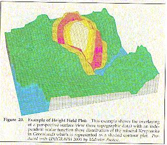
An example of a height-field plot produced in IRIS Explorer.

Multiple Scalar Fields: E^mS₂

At each point, the values are represented by some sort of icon, that can vary in size, shape, color, sound, etc.

Scalar Field using Lighting and Shading: E^S₂

This would be a scalar field defined over a geometric surface, such as temperature over an aircraft wing surface. The geometric surface would be defined as polygons or by parametric cubic curves. Light sources and Gouraud or Phong shading can be used to enhance the 3D effect. Note that this is categorized as E^S₂ since the geometric surface can be defined as patches in 2D parametric space.

Bounded Region Plot: E^S_[2]

The entity to be displayed is defined over a set of regions, e.g., population density over counties. Click here for an example of a bounded region plot.

Visualization Techniques for Data Display
HyperVis Table of Contents